| Inkscape » Extensions » Render |    |
|---|
| Inkscape » Extensions » Render | |
|---|
This set of extensions creates new objects.
This extension generates 3D Polyhedrons. Selecting this extension pops up a dialog with three tabs. The first tab, Model file, controls the type of polyhedron that is specified in the Object drop-down menu. If Load From file is selected, the description in the file specified in the Filename: entry box is used. In the Object Type tab you can specify if the source file describes the object with edges or faces.

The second tab, View, allows you to rotate the polyhedron. Up to six rotations are allowed (for the mathematicians: why six when any unique rotation can be specified by only three orthogonal rotations?).

The third tab, Style, allows you to set all kinds of style parameters, including the Fill color and opacity. One can also specify if the faces of the polyhedron should be shaded to simulate light striking the object. One can specify the direction from which the light comes. One can specify if the nodes, edges, or faces should be drawn. And one can specify if the “hidden” faces should be drawn (useful if the faces are not fully opaque).


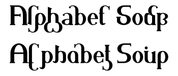
This extension generates exotic-looking text by recombining parts of characters from mostly the Latin alphabet in a way that the original text is discernible. The dialog has entry boxes for the text, scale, and random number seed. Changing the random number seed will change the parts used to generate the text. This effect is based on code written by Matt Chisholm.
This extension generates barcodes. The types of codes that can be generated are:

New in v0.48.
This extension generates a Datamatrix barcode.

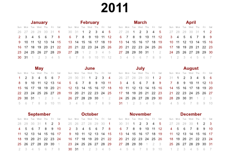
This extension generates calendars. There are a variety of options. One can select a whole year or one month. One can choose Sunday or Monday as the starting day of the week, and one can choose which days are considered to be weekend days. One can choose the colors for the different labels and one can change the default names of the months and the days of the week.
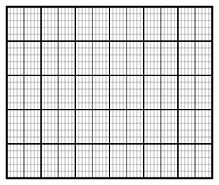
This extension generates Cartesian grids. Options include number of subdivisions, number of sub-subdivisions, linear versus logarithmic divisions, and line widths. For polar coordinates see Polar Grid extension.
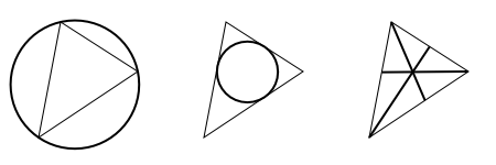
This extension is a geometrician's dream. It allows you to create an almost infinite number of constructions based on a triangle. The triangle is defined by the first three nodes in a path (even if the path is not a triangle). The path must be closed and the nodes connected by straight lines.
This extension draws the pattern for a foldable box as one might use for the input in a desktop cutting plotter (after modifying the paths). The individual sides and tabs are each represented by separate paths which are all in a Group.

Plot a function versus x (horizontal axis). To use, first draw a rectangle to define the width of the x-axis and the height of the ±1 lines of the y-axis. Then select the extension. In the pop-up window, enter the x and y ranges. Checking the Multiply x-range by 2π box changes the x-axis to represent units of 2π, useful for plotting periodic functions. You can either have the routine calculate the first derivative of the function numerically or supply the first derivative yourself.
The function is plotted in the SVG coordinate system, which has the y-axis upside down. The extension inserts a minus sign automatically to correct for this.
All Python math functions are allowed (as long as they return a single value), including Python random number functions. The Help Tab has a list of some of the available functions.

When the Use polar coordinates option is selected, the x-range is set to −1 at the left of the rectangle and +1 at the right side. The x values entered in the extension's dialog are used for the angle domain (in radians). The Isotropic scaling parameter is ignored. Calculate first derivative numerically must also be selected.

Note that depending on the version, Python may return an integer if you divide two integers: thus, 4/5 = 0, while 4.0/5.0 = 0.8.
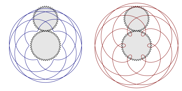
Draw a realistic mechanical gear. Three parameters must be given: the Number of teeth, the Circular pitch (the tangential distance between successive teeth), and the Pressure angle. Common values for Pressure angle are: 14.5, 20, and 25 degrees. The radius of the “Pitch Circle” is equal to N × P/2π, where “N” is the number of teeth and “P” is the Circular Pitch.
The gear is created around the SVG origin and then placed inside a Group. The Group is then translated so that the center of the gear is at the center of the visible canvas. This makes animating the gear easier as the rotation is then independent of the displacement. An animated clock using these gears can be found on the book's website.

This extension fills the bounding box of an object with a grid. The grid spacing and offset can be independently set in the horizontal and vertical directions. The grid line width can also be set.
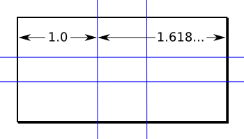
This extension creates Guide Lines based on the Page size. One can choose between three Preset options. The first option, Custom..., allows one to create evenly spaced Guide Lines with the spacing defined by the Vertical guide each and Horizontal guide each menus. The next Preset option, Golden Ratio, places Guide Lines so that the ratios horizontally or vertically from the Guide Lines to the edges of the page are in proportion to the Golden Ratio (approximately 1 to 1.62). The last Preset option, Rule-of-third, divides the Page horizontally and vertically into three equal parts. This is equivalent to using the Custom... option with a value of 1/3.
Enabling the Start from edges option will result in Guide Lines also being created along the Page edges.
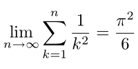
This extension turns a LaTeX string into a path. The string is typed into a dialog box. The extension requires that Ghostscript, LaTeX, and Pstoedit to be installed and in the execution path. Pstoedit must include the GNU libplot SVG driver or the shareware SVG plug-in, available for Windows at the Pstoedit website. The resulting formula is rendered as a path.
An alternative script for Linux using Skencil for the conversion to SVG (avoiding the need for Pstoedit with SVG support) is available at the book's website: http://tavmjong.org/INKSCAPE/.
Draws Lindenmayer System structures, developed by Aristid Lindenmayer while studying yeast and fungi growth patterns. It is beyond the scope of this manual to discuss these structures. Just one comment: The Step parameter controls the scale of the generated path.

Lindenmayer Systems: From left to right:
Default inputs.
Variant of the Koch curve. Inputs: Order 3, Angles 90, Axiom F, Rules F=F+F-F-F+F.
Koch's Snowflake: Inputs: Order 3, Angles 60, Axiom F++F++F, Rules F=F-F++F-F.
Sierpinski triangles. Inputs: Order 5, Angles 60, Axiom A, Rules A=B-A-B;B=A+B+A.
The rules can be very complex. See the Lindenmayer screenshot for more information.
This extension generates parametric curves. It was derived from the Function Plotter extension and shares many of its parameters.

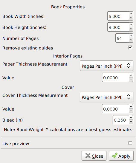
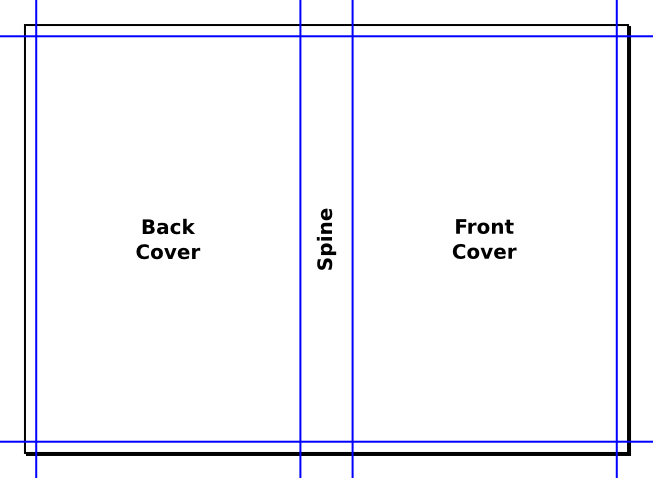
This extension produces a template for a Perfect-Bound Cover as found in Print On Demand services. The template sets the document to the correct size and creates guides for the front cover, back cover, and spine of the book, including the specified bleed. The dialog allows for specifying a variety of parameters including the number of pages in the book and the thickness of each page. The extension is biased toward English measurements.
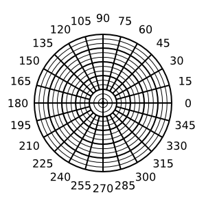
This extension generates polar grids. Options include number of subdivisions, linear versus logarithmic divisions, line widths, and angle labels. For Cartesian coordinates see Cartesian Grid extension.
This extension generates printing marks. Options include generating crop marks, bleed marks, registration marks, star target, color bars, and page information. At the moment, the marks are generated “off” the page. The Selection option in the Set crop marks to drop-down menu in the Positioning tab does not work. You will have to enlarge the Page and translate the drawing with marks after applying this extension. Note that the printing marks are created on a locked Layer named Printing Marks.


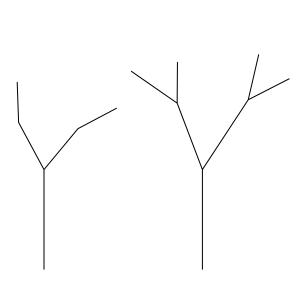
Draw a random tree made of straight-line segments. This is a classic from Turtle Geometry. This implementation is rather limited.
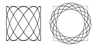
Draw a Spirograph; that is, an epitrochoid or hypotrochoid curve. Several parameters need to be given: “R”, the Ring Radius; “r”, the Gear Radius; and “d”, the Pen Radius. In addition, one must choose if the Gear travels Inside or Outside the Ring. One can also set the Rotation angle (the angle of the starting point relative to the center) and the Quality (roughly, the number of nodes per loop).

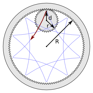
The ratio of “r” to “R” determines the structure of the curve. Take, for example, an “r” of 36 and an “R” of 48. The ratio reduced to its simplest form is 3/4. This indicates that the Gear will make a total of four “loops” as it circles the Ring three times. Simple ratios make simple curves. If you use an Even-odd fill rule, the center of the figure will be unfilled if the denominator is even.
Unlike the case with a real Spirograph that utilizes plastic gears, it is possible to specify values of “r” and “R” that don't form a rational number ratio. In this case, the curve never closes on itself and is of infinite length. To avoid such infinities, the extension limits the number of nodes to 1000. If the numerator or denominator of the ratio in the simplest form is a large integer, the Spirograph may run out of nodes. In this case, decreasing the Quality may help.

Also, unlike a “real” Spirograph, the Spirograph extension allows “d” to be greater than “r”. This results in small loops along the Ring.
This extension generates triangles. Although there are six parameter entry boxes, only three are used at any one time. Which three are used is specified in the Mode drop-down menu. Side c is always at the bottom.

New in v0.48.
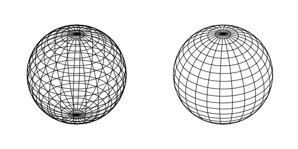
This extension generates a wire frame sphere using ellipses to represent lines of latitude and longitude. The number of lines can be specified as well as the orientation of the sphere. An option allows the removal of hidden lines.
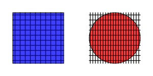
| |  | |
| Raster |  | Text |
© 2005-2017 Tavmjong Bah. |  |